Performance Optimisation and Productivity
Finite Difference Methods
Finite different methods (FDM) is a general numerical method for solving ordinary differential equations (ODE) or partial differential equations (PDE) raising from approximating (non-)linear physical and mathematical problems. The original differential equation is solved on a grid of points where finite difference formulas are used to approximate the solution using the surrounding values. This way, we can transform a differential equation into a system of algebraic equations to solve.
Taylor’s expansion of a one-dimensional function \(f(x)\) on an \(h\)-surrounding of a point \(x_0\) can be written as
\[f(x_0 + h) = f(x_0) + \frac{f'(x_0)}{1!} h + \frac{f''(x_0)}{2!}h^2 + ...\]From applying that series to \(f(x_0 - h)\) and \(f(x_0 + h)\), we can derive the second order centered difference approximation of \(f'(x)\) and \(f''(x)\),
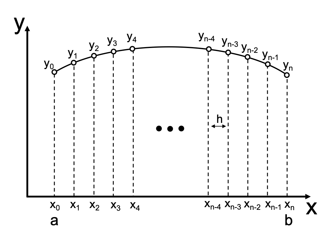
\[\frac{dy}{dx} = \frac{y_{i+1} - y_{i-1}}{2h}, \\ \frac{d^2y}{dx^2} = \frac{y_{i-1} - 2y_i + y_{i+1}}{h^2}.\]The corresponding figure shows the interval of \([a,b]\) that is equally divided into subintervals of length \(h\).
Here, we present central finite differences as they are the most common and straightforward. In general, various methods may be used, depending on the required accuracy and computational costs — E.g., forward or backward finite differences or higher-order finite differences. The same idea is applicable for multidimensional problems with both spatial and time dimensions. Finite difference formulas are derived from the Taylor series. The approximation error is given by the regularity of the original function and the used order (number of elements in Taylor expansion).
The basic principle lies in converting a solution of an ordinary differential equation (ODE) problem or a partial differential equation (PDE) problem into a solution of a system of linear algebraic equations \(Au=f\), where A is a sparse system matrix (e.g., stiffness matrix, thermal conductivity matrix, etc.), u is a vector of unknown state variables (e.g., displacements, temperatures, etc.) in domain mesh nodes, and \(f\) is a known right-hand side vector (e.g., external forces, heat sources, etc.).
EXAMPLE: (simple one-dimensional problem)
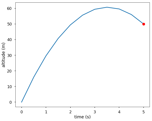
We are going out to launch a rocket, and let \(y(t)\) is the altitude (meters from the surface) of the rocket at time \(t\). We know the gravity \(g=9.8m/s2\). If we want to have the rocket at 50 m off the ground 5 seconds after launching, what should be the launch velocity? (we ignore the drag of the air resistance). We solve the rocket problem using the central finite difference method and plot the altitude of the rocket after launch.
The related ODE is
\[\frac{d^2y}{dt^2} = -g,\]with the boundary conditions \(y(0)=0\) and \(y(5)=50\). Let’s take \(n=10\).
Since the time interval is \([0,5]\) and we have \(n=10\), therefore, \(h=0.5\), using the central finite differences as the approximation for derivatives, we have
\[y_0 = 0, \\ y_{i-1} - 2y_i + y_{i+1} = -gh^2, i=1,2,...,n-1 \\ y_{10} = 50\]if we use matrix notation, we will have:
\[\begin{bmatrix} 1 & 0 & & & \\ 1 & -2 & 1 & & \\ & \ddots & \ddots & \ddots & \\ & & 1 & -2 & 1 \\ & & & & 1 \end{bmatrix}\begin{bmatrix} y_0 \\ y_1 \\ \vdots \\ y_{n-1} \\ y_n \end{bmatrix} = \begin{bmatrix} 0 \\ -gh^2 \\ \ldots \\ -gh^2 \\ 50 \end{bmatrix}\]Therefore, we have 11 equations in the system. A solution to this problem is implemented in the following python code.
import numpy as np
import matplotlib.pyplot as plt
plt.style.use('seaborn-poster')
%matplotlib inline

n = 10
h = (5-0) / n

# Get A
A = np.zeros((n+1, n+1))
A[0, 0] = 1
A[n, n] = 1
for i in range(1, n):
    A[i, i-1] = 1
    A[i, i] = -2
    A[i, i+1] = 1

print(A)

# Get b
b = np.zeros(n+1)
b[1:-1] = -9.8*h**2
b[-1] = 50
print(b)

# solve the linear equations
y = np.linalg.solve(A, b)

# graphical output
t = np.linspace(0, 5, 11)

plt.figure(figsize=(10,8))
plt.plot(t, y)
plt.plot(5, 50, 'ro')
plt.xlabel('time (s)')
plt.ylabel('altitude (m)')
plt.show()