Finite Element Method

Finite Element Method (FEM) is a general numerical method for solving physical problems in engineering analysis and design. It is used for modelling of a continuum in steady-state, propagation (transient), and eigenvalue problems in many domains, e.g. structural mechanics, CFD, thermodynamics, electromagnetics, etc. It is a robust universal method able to solve large complex systems for the price of relatively high computational demands.

The basic principle lies in converting a solution of a partial differential equation (PDE) problem into a solution of a set of systems of linear algebraic equations \(Au=f\), where \(A\) is a sparse system matrix (e.g., stiffness matrix, thermal conductivity matrix, etc.), \(u\) is a vector of unknown state variables (e.g., displacements, temperatures, etc.) in domain mesh nodes, and \(f\) is a known right-hand side vector (e.g., external forces, heat sources, etc.). The FEM then calculates an approximate (numerical) solution of the original problem with a given precision.

The solution of a particular physical problem using the FEM requires the following steps:

1. System idealization and definition of a mathematical continuum-system model, material parameters, boundary conditions, etc.
2. Creation of a mesh of finite elements of the continuum-system model using a discretization method
3. Assembling of local FEM systems per element
4. Assembling of the global FEM system
5. Incorporation of boundary conditions
6. Solving of the FEM system using some direct or iterative sparse linear-system solver
7. Interpretation of results

A working example of a FEM solution of a 1D static (time-invariant) model that can represent e.g. heat transfer, diffusion, linear elasticity etc. In MATLAB follows:

where \(k\) is a material function defining material properties, \(u\) is an unknown function (quantity, e.g. temperature), \(f\) is a known scalar function (e.g. source term), \(\Omega\) is a domain of a problem given by a range between \(0\) and \(l\), \(\hat{u}\) is a given value of the solution \(u\) in the point \(0\) (Dirichlet boundary condition), and \(\hat{\tau}\) is a given value corresponding to the derivative of the solution \(u\) in the point \(l\) (Neumann boundary condition).

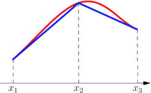
The graph shows an exact smooth solution (red curve) and its piecewise linear approximation using the FEM (blue curve).

%----------------------------------------------------%
%                  FEM 1D                            %
%----------------------------------------------------%
function FEM1D 
% Input data
x = 0 : 1/2 : 1; % nodes coordinates
el = [1, 2; 2, 3]; % element nodes (element per row) 
k = [1, 1]; % material coeffs
f = [0.75, 0.25]; % sources in elements
bc = [0, 1, 2; 1, 3, 0.25]; % boundary conditions in format [type (0-Dirichlet/1-Newton), node, value] per row
n = length(x); % num of nodes
nel = size(el, 1); % num of elements

% Assembling of local FEM systems
Ael = [1, -1; -1, 1];
bel = [1; 1];

% Assembling of global FEM system
A = zeros(n, n);
b = zeros(n, 1);
for i = 1 : nel 
    A(el(i, :), el(i, :)) = A(el(i, :), el(i, :)) + (k(i) / (x(el(i, 2)) - x(el(i, 1)))) * Ael; 
    b(el(i, :)) = b(el(i, :)) + (0.5 * f(i) * (x(el(i, 2)) - x(el(i, 1)))) * bel;
end

% Incorporation of boundary conditions
for i = 1 : 2
    if bc(i, 1) == 1
        b(bc(i, 2)) = b(bc(i, 2)) + bc(i, 3);
    end
    if bc(i, 1) == 0
        b = b - bc(i, 3) * A(:, bc(i, 2));
        A(:, bc(i, 2)) = zeros(n, 1);
        A(bc(i, 2), :) = zeros(1, n);
        A(bc(i, 2), bc(i, 2)) = 1;
        b(bc(i, 2)) = bc(i, 3);
    end
end

% Solving of the FEM
u = A \ b

% Graphical output
plot(x, u, '-ob', 'LineWidth', 2, 'MarkerEdgeColor', 'k', 'MarkerFaceColor', 'g', 'MarkerSize', 10);
hold on; grid on;
title(texlabel('FEM 1D'), 'FontSize', 14);
xlabel(texlabel('x'), 'FontSize', 14);
ylabel(texlabel('u(x)'), 'FontSize', 14);