Performance Optimisation and Productivity
Tuning BLAS routines invocation
Speedup plots
A simple code was used to identify the best block partitioning of matrix multiplication when splitting \(\bf{A}\) over the rows and \(\bf{B}\) over the columns, where all processes have access to \(\bf{B}\) and \(\bf{A}\). For this purpose, it is not necessary to implement the actual algorithm, it is sufficient to measure the time taken for representative computation on a single compute node.
The sequential dgemm subroutine from MKL-2017 is used to perform each block multiplication. The three matrices have size \(N_n \times N_n\) where \(N_n = 3600\). The data below is for a fully loaded compute node on MareNostrum-4, i.e. 48 processes per node, and the computation on each process is repeated 100 times to give measurable timings. Figure 1 shows the speedup plot for \(N_w=N_n/(2 \times nNodes)\) and \(N_v=N_m/24\), with \(nNodes=1,2,4,6\).
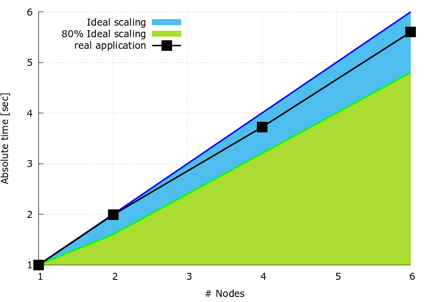
Figure 1: Speedup plot.
It can be observed that the splitting of both matrices and a careful selection of the block size improve significantly the speedup of the code wrt the pattern case. In fact, in all cases, the speedup is always higher than \(80 \%\) ideal.
PAPI counters
To compute the IPC, the total number of instructions (PAPI_TOT_INS) and total number of cycles (PAPI_TOT_CYC) have been collected from rank 0.
In Table 1, the IPC for 1,2,4,6 nodes are shown using the same parameters as for the speedup tests.
| number of nodes | timing [sec.] | PAPI_TOT_INS | PAPI_TOT_CYC | IPC | IPC Scaling | Instruction Scaling | Frequency Scaling | Computaion Scaling |
|---|---|---|---|---|---|---|---|---|
| 1 | 4.31 | 21,904,606,763 | 8,283,930,507 | 2.64 | 1.00 | 1.00 | 1.00 | 1.00 |
| 2 | 2.17 | 10,962,982,391 | 4,129,727,218 | 2.66 | 1.01 | 1.00 | 0.99 | 1.00 |
| 4 | 1.16 | 5,491,864,214 | 2,045,283,168 | 2.68 | 1.01 | 1.00 | 0.92 | 0.93 |
| 6 | 0.77 | 3,662,517,229 | 1,356,691,163 | 2.65 | 1.00 | 1.00 | 0.92 | 0.92 |
Table 1: IPC, timing, PAPI counters and scaling values for \(N_w=N_n/(2 \times nNodes)\) and \(N_v=N_m/24\), with \(nNodes=1,2,4,6\).
The IPC is much higher with respect to the one observed for the pattern and it shows what a better partitioning strategy can do to speed up the block’s multiplication. To investigate more the IPC to performance relationship, the whole combination of \(N_w/n_{parts}\) and \(N_v/m_{parts}\), with \(n_{parts}\) and \(m_{parts}\) integers, is reported in Figure 2.
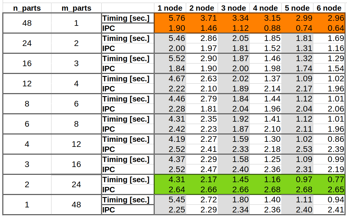
Figure 2: IPC values and timing for different combination combination of \(N_w=N_n/n_{parts}\) and \(N_v=N_m/m_{parts}\) values.
In this test, \(N_m\) and \(N_n\) are fixed while the number of blocks for the columns and rows are changed by using two parameters \(n_{parts}\) and \(m_{parts}\), namely, \(N_w=N_n/n_{parts}\) and \(N_v=N_m/m_{parts}\). Moreover, the product of the two is equal to the total number of processes over all nodes.
It can be observed how the overall best performance (green row) is obtained when, on one node, \(N_w=N_n/2\) and \(N_v=N_m/24\) with an average IPC constant and around \(2.65\) for all the node counts. In comparison, the pattern (red row), achieves a very poor performance in terms of timing and IPC. Other cases, such as \(N_w=N_n/8\) and \(N_v=N_m/6\), show good IPC and timing, different configuration can give similar performance.
 )
)
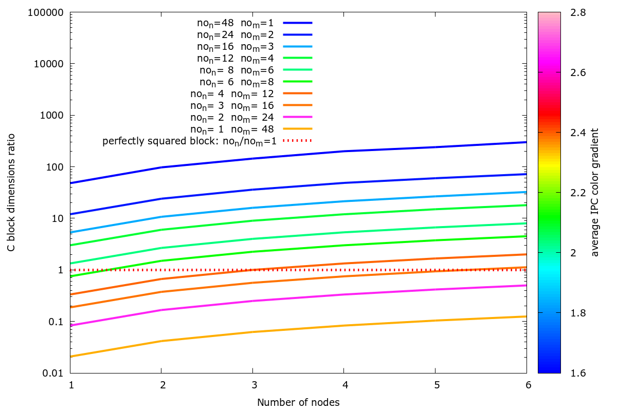
Figure 3: \(N_w/N_v\) ratio versus node counts. Combinations of \(N_w/N_v\) with high IPC are coloured in red/pink.
In Figure 3, the \(N_w/N_v\) ratio versus the number of nodes is shown. The horizontal line marks a perfectly squared block (i.e. \(N_w/N_v=1\)), the colour of each line is computed by using the average IPC over the runs, combinations with high IPC are coloured in red/pink while combinations with low IPC are coloured in blue/green. The combinations with the highest IPC are all nearby the \(N_w/N_v=1\) horizontal line.