Low computational performance calling BLAS routines

Speedup plots

A simple benchmark code is used to measure parallel scaling matrics for the pattern. The computation is repeated 100 times (n_rep=100) to give measurable timings. The three matrices have size \(N_n \times N_n\) where \(N_n = 3600\), and the number of simulated nodes vary from one to six.

The data in Figure 1, is for a fully loaded compute node on MareNostrum-4, i.e. \(48\) processes per node. The speedup plot is obtained using a sequential version of dgemm subroutine from MKL-2017.

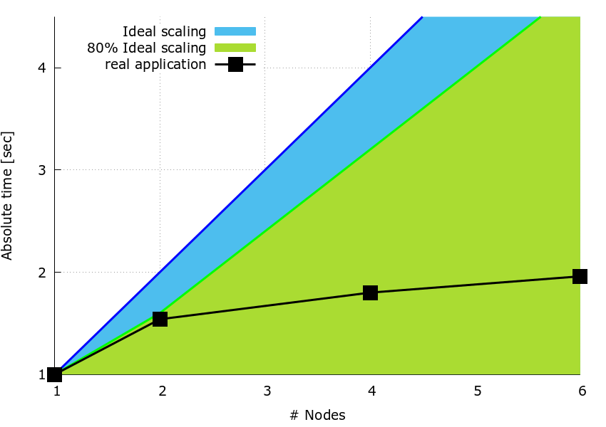
Figure 1: Speedup plots.

It can be observed that partitioning the work by slitting matrix \(\bf{B}\) over the columns results in a reduced speedup when the number of nodes increases (e.g. \(<30\%\) on 6 nodes).

PAPI counters

PAPI counters are used to verify that it is IPC scaling which causes the drop in performance. To compute the IPC, the total number of instructions (PAPI_TOT_INS) and total number of cycles (PAPI_TOT_CYC) have been collected from rank 0.

In Table 1, the IPC for 1,2,4,6 nodes are shown using the same parameters as for the speedup tests.

number of nodes	timing [sec.]	PAPI_TOT_INS	PAPI_TOT_CYC	IPC	IPC Scaling	Instruction Scaling	Frequency Scaling	Computaion Scaling
1	5.76	21,290,936,337	11,252,982,643	1.90	1.00	1.00	1.00	1.00
2	3.71	10,541,309,910	7,246,701,160	1.46	0.59	0.99	1.00	0.76
4	3.15	5,372,521,162	6,099,643,964	0.88	0.46	1.01	1.01	0.46
6	2.96	3,589,459,236	5,648,445,982	0.64	0.34	1.01	1.01	0.33

Table 1: IPC, timing and PAPI counters for the pseudo-code application.

A significant drops in IPC can be observed when moving from one to 6 nodes. The IPC scaling is low aleady on 2 simulated nodes (i.e. \(0.59\)) and it keeps reducing significantly up to 6 nodes (i.e. \(0.34\)). Instruction and Frequency scaling are both optimal. The Computation scaling is poor from two to six simulated nodes due to the poor IPC scaling.

Different version of MKL (i.e.: MKL-2021 and OpenBLAS) have been tested, similar results hold in both cases.