Performance Optimisation and Productivity
OpenMP collapse loops experiments
The data reported below are for strong scaling experiments. The runs have been performed on MareNostrum 4, with one node and up to 48 threads.
The code snippet executed for the no-collapse case is
DO iter = 1, Niter
    !$OMP PARALLEL DO DEFAULT(NONE) SHARED(...)
    DO K = 1, Nk
        DO J = 1, Nj
            DO  I = 1, Ni
                !! work to do
            END DO
        END DO
    END DO
    !$OMP END PARALLEL DO
END DO
While the code snippet executed for the COLLAPSE(2) case is
DO iter = 1, Niter
    !$OMP PARALLEL DO COLLAPSE(2) DEFAULT(NONE) SHARED(...)
    DO K = 1, Nk
        DO J = 1, Nj
            DO  I = 1, Ni
                !! work to do
            END DO
        END DO
    END DO
    !$OMP END PARALLEL DO
END DO
For the COLLAPSE(2) case, the K and J loops are fused by the compiler to create a single iteration space of dimension Nk*Nj , which can improve the distribution of work over the threads when Nk is small.
Speedup plots
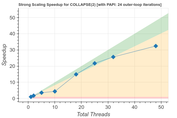
In Figure 1, the speedup plots for the no-collapse case and the COLLAPSE(2) case are shown, for the case Nk=22, Nj=42, Ni=82, and Niter=24.
| COLLAPSE(2) case | no-collapse case |
|---|---|
 |
 |
Figure 1: Speedup plots for the no-collapse case and the COLLAPSE(2) case.
The speedup for the COLLAPSE(2) case is improved compared to the no-collapse case, and for most threads counts is close to optimal (e.g. >80%).
POP Metrics
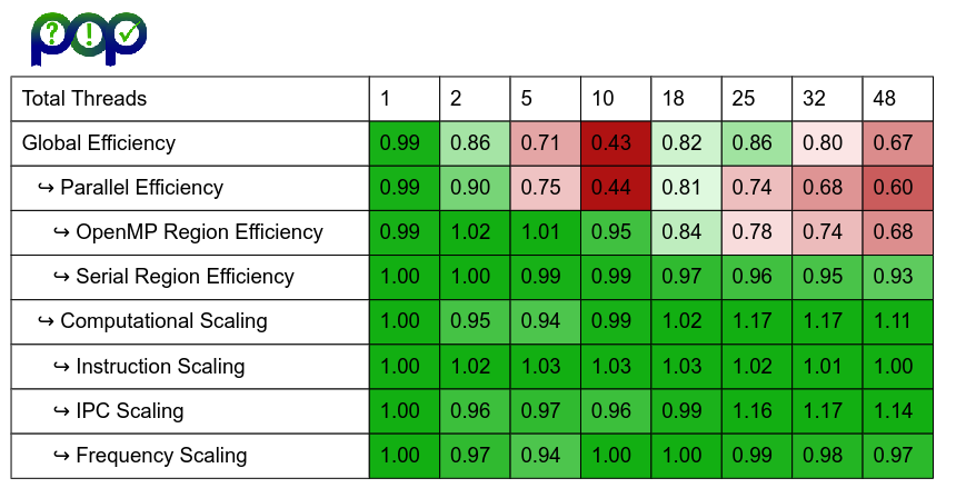
Figure 2 shows POP OpenMP metrics for the no-collapse and COLLAPSE(2) cases, for the same case as the speedup plot above. A full description of the POP OpenMP metrics can be found in the Hybrid Metrics here. The important metric to understand here is OpenMP efficiency, which measures the efficiency of the OpenMP regions, including the efficiency of the load balance within the OpenMP regions. Parallel Efficiency and Global Efficiency are also impacted by low efficiency within OpenMP.
The POP metrics for both cases are similar, other than OpenMP Efficiency, Parallel Efficiency and Global Efficiency. From 18 threads onwards for the no-collapse case there are significantly low values for OpenMP Efficiency, whereas the COLLAPSE(2) case shows good efficiency values.
| COLLAPSE(2) case | no-collapse case |
|---|---|
 |
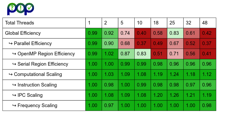 |
Figure 2: POP OpenMP metrics for the no-collapse case and the COLLAPSE(2) case.
Tracefiles
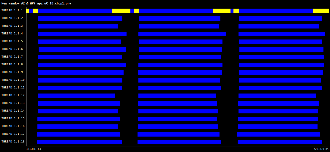
In Figure 3, Extrae timeline windows for the no-collapse case and the COLLAPSE(2) case are shown. The Extrae timeline windows show three iteration of the nested parallel loop for 18 threads. The code executed inside the inner loop is the same for all values of I. As it can be observed, the no-collapse case shows a significant imbalance of computation.
| COLLAPSE(2) case | no-collapse case |
|---|---|
 |
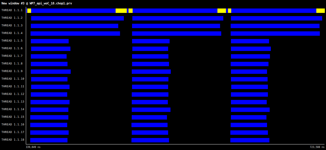 |
Figure 3: Timeline view for the no-collapse case and the COLLAPSE(2) case. The parameters used for these runs are Nk=22, Nj=42, Ni=82, and Niter=24.
Run-time plots
One last experiment measures the run-time of the two cases, shown in Figure 4. For the propose of the benchmark, the timing has been computed starting from the second iteration of the parallel loop (i.e. Niter=2) by using the omp_get_wtime() routine. The parameters used for these runs are Nk=4, Nj=50, Ni=1640, and Niter=250. From 5 threads onwards the COLLAPSE(2) case shows significantly faster execution than the no-collapse case.
| COLLAPSE(2) case (blue) vs no-collapse case (green) |
| —— |

Figure 4: Absolute run-time plots for the no-collapse case and the COLLAPSE(2) cases. The parameters used for these runs are Nk=4, Nj=50, Ni=1640, and Niter=250.