Tuning BLAS routines invocation (gemm)

In many scientific applications, parallel matrix-matrix multiplications represent the computational bottleneck. Consider the following matrix-matrix multiplication:

where, \(\bf {A}\) is a matrix with \(N_m\) rows and \(N_k\) columns (i.e. \(N_m \times N_k\)), \(\bf {B}\) is a \(N_k \times N_n\) matrix so that \(\bf {C}\) is a \(N_m \times N_n\) matrix.

In the case each process has access to \(\bf {A}\) and \(\bf {B}\), a strategy to parallelise the work is to divide \(\bf {A}\) and/or \(\bf {B}\) into blocks to partition the computation over all processes, and use BLAS routines, e.g. dgemm, on the individual block multiplications. 

It can be observed that different partitioning of the matrices \(\bf {A}\) and \(\bf {B}\) can result in different computational performance due to different values of IPC (instructions per cycle). For example, splitting \(\bf {B}\) over the columns and leaving \(\bf {A}\) unchanged can result in poor computational scaling (see the related pattern addressed).

When such poor parallel scaling occurs, it is best practice to write a simple code in order to test alternative partitioning of the matrix multiplication. In the case described above, where \(\bf {B}\) is split over the columns, and \(\bf {A}\) is not split, the size of the matrix blocks is determined by the number of processes. However, if we split \(\bf {A}\) over the rows, whilst still splitting \(\bf {B}\) over the columns, we have a choice of the size of the matrix blocks for \(\bf {A}\) (i.e. \(N_v=N_m/n_{parts_A}\)) and of \(\bf {B}\) (i.e. \(N_w=N_n/n_{parts_B}\)), where \(n_{parts_A}\) and \(n_{parts_B}\) are two integers and their product would typically equal the number of processes.

The calculation of a block of matrix \(\bf {C}\), defined as \(\bf {C_{v,w}}\) with size \(N_v \times N_w\), can be expressed as:

By experimenting with blocks of \(\bf {C_{v,w}}\) having different values of \(n_{parts_A}\) and \(n_{parts_B}\), namely different values for columns (\(N_w\)) and rows (\(N_v\)), we can find out optimal pairs.

The pseudo-code implementation of the aforementioned algorithm can be:

  given:
   N_m, N_n, N_k, n_parts_B

  execute:
   get_my_process_id(proc_id)
   get_number_of_processes(n_proc)

   DEFINE first_b, last_b, len_n_part AS INTEGER
   DEFINE first_a, last_a, n_parts_A, len_m_part AS INTEGER
   DEFINE alpha, beta AS DOUBLE

   first_b = float(N_n) * proc_id / n_parts_B
   last_b = (float(N_n) * (proc_id + 1) / n_parts_B) - 1

   n_parts_A = n_proc / n_parts_B

   first_a = float(N_m) *  proc_id / n_parts_A
   last_a = (float(N_m) * (proc_id + 1) / n_parts_A) - 1

   len_n_part = last_b - first_b + 1;
   len_m_part = last_a - first_a + 1;

   SET alpha TO 1.0
   SET beta TO 0.0
   call dgemm('N', 'N', len_m_part, len_n_part, N_k, alpha, A[:,first_a:last_a], len_m_part, B[:,first_b:last_b], N_k, beta ,C, len_m_part)

Speedup tests

The speedup plot below is from a simple timing code written to test the strategy of dividing both matrices, \(\bf{B}\) and \(\bf{A}\), into blocks, and splitting the individual multiplications over the processes using the sequential dgemm subroutine from MKL-2017. The code doesn’t actually implement the parallel matrix-matrix multiplication, it simply replicates the same computation for one node. The proposed best-practice is meant to show how a simple code can be used to compare the timing for different splitting on \(nNodes\) nodes relative to one node and to identify the best partition.

The three matrices have size \(N_n \times N_n\) where \(N_n = 3600\). On one node, the number of columns for \(\bf{B_w}\) is \(N_w=N_n/ (2 \times nNodes)\) while the number of rows of \(\bf{A_v}\) is \(N_v=N_m/24\) for all cases.

The speedup plot in Figure 1, is obtained by using the sequential dgemm with parameters alpha and beta are set to \(1.0\) and \(0.0\), respectively.

The code was run on a fully populated compute node of MN4 i.e. using 48 processes, the computation was repeated \(100 \times\) to give measurable timings.

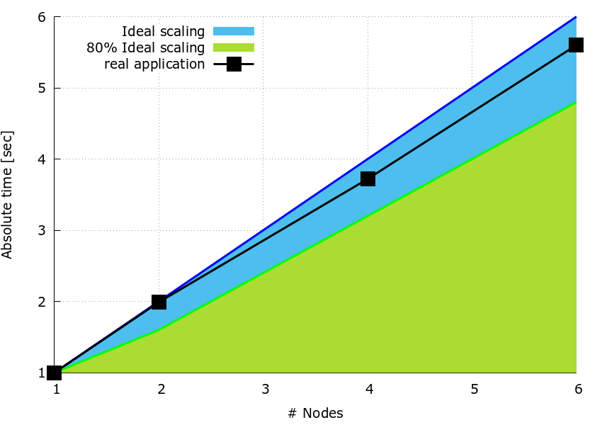Figure 1: speedup plot.

In contrast to the pattern, it can be observed how the speedup of each run is always higher than \(80 \%\) with respect to the ideal.