Poor GPU data transfer rate due to affinity

Most CPUs are organized in multiple NUMA domains. Accessing different parts of the memory from a certain core of such a CPU therefore has different performance. We call this affinity. Since each available GPU on a system is connected to a NUMA domain this effect also is observable in data transfers from and to the GPU. Depending on the location of the data on the host side and the core that is handling the data transfer, both bandwidth and latency can vary significantly.

The following code implements the commonly used saxpy operation calculating \(aX+Y\) with the vectors $X$ and $Y$ and a scalar factor $a$. It uses OpenMP target offloading to run the code on the GPU:

void saxpy(size_t n, float a, float* x, float* y, float* r){
    #pragma omp target device(d) map(to:x[0:n]) map(to:y[0:n]) map(from:r[0:n])
    {
        #pragma omp teams distribute parallel for 
        for(int k = 0; k < n; ++k) {
            r[k] = a * x[k] + y[k];
        }
    }
}

The code transfers data to the GPU, does a simple calculation and transfers the result back. With a sufficiently large input the runtime of this function differs significantly. The runtime depends on where the host data is allocated and which core/device combination is used to handle the data transfer. The following plot shows the runtime for different core/device combination on a 2x48 core system with 4 GPUs. The size of the vectors x and y used in the saxpy is 400 MB. The result r copied back also has the size 400MB.

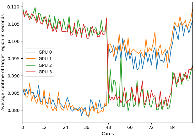
The results correspond to the sockets that are present on the system:

• GPU 0 is connected to NUMA node 0 (socket 0, cores 0-11)
• GPU 1 is connected to NUMA node 2 (socket 0, cores 24-35)
• GPU 2 is connected to NUMA node 4 (socket 1, cores 48-59)
• GPU 3 is connected to NUMA node 6 (socket 1, cores 72-84)

The runtimes heavily differ between the sockets used to handle the data transfer to the GPU. The computation done inside the target region is the same for all the runs performed, the difference in runtime only comes from the difference in the transfer speeds to the GPU.

Information about the GPU configuration can be obtained with various tools like nvidia-smi or rocm-smi.

Choosing the correct cores for initializing data and transfering it to the GPU can have an impact on the performance of a code. This problem becomes more significant when using large data where the data transfer takes more time.

The difference in bandwidth can manifest as a load balance issue. Consider the following code pattern:

for(int i = 0; i < n_steps; ++i){
    saxpy(...); // some function including GPU copies and computation
    MPI_Barrier(MPI_COMM_WORLD);
}

If we launch one MPI rank per available GPU without specifying where the MPI ranks should run, the trace of such an application may look like this trace.

We can see that the first process finishes faster even though the computational load is the same. This is due to the faster CPU to GPU transfers that are available on rank 0 as it was executed on the NUMA domain the used GPU is connected to. However, rank 2 and 3 execute on socket 0 while the used GPUs 2 and 3 are connected to socket 1. This heavily increases the runtime and results in a load imbalance. The resulting MPI Load Balance Efficiency is 86%.